
|
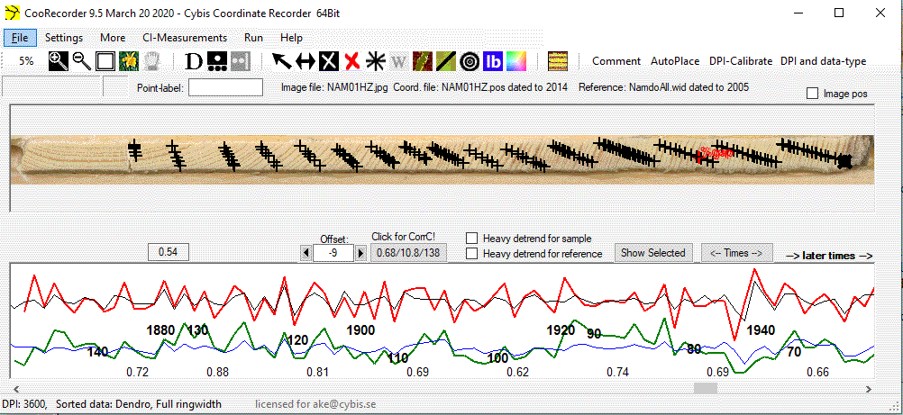
This is NAM01 - a sample from a Scots pine growing on the island of Nämdö. Soxhlet treating, sanding and polishing and scanning was managed by Ryszard J. Kaczka and Karolina Janecka. The soxhlet treatment is evident from the light surface. The brown tar has apparently been removed through the soxhlet process. For the sample NAM01 we have an image file NAM01HZ.jpg and also a .pos file "NAM01HZ.pos" with position coordinates. The measurements in the .pos file have been done in CooRecorder with a reference curve (a mean value curve) as a necessary support as there is a big number of false or almost missing rings in NAM01HZ. A suitable reference is NamdoAll.wid. You can also create your own reference from the ITRDB swed302.rwl collection.It is practical to save copies of these three files in a separate directory with a short path, e.g. C:\_BLUES\_BLUEWID\ or C:_BLUES\NAM01\ or alike to have the files easily available for crossdating experiments.
|
|
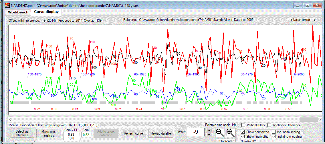
The NAM01 red and green curves will now overlay the reference curves. If they are not in synchronized position, click the "Click for CorrC!" button above the curve diagrams.
Click the "Fit on screen" icon at the top of the screen to make the image somewhat larger. You should now see something as shown above.
We are now set up for collecting some blue data! |
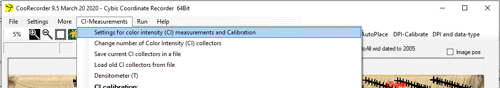
| Click the menu command "CI-measurements/Settings for color intensity (CI) measurements and calibration" |
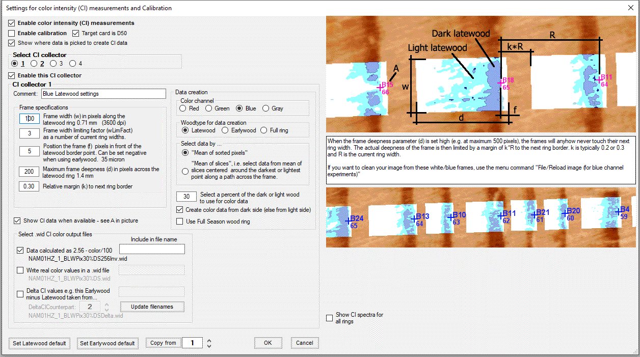
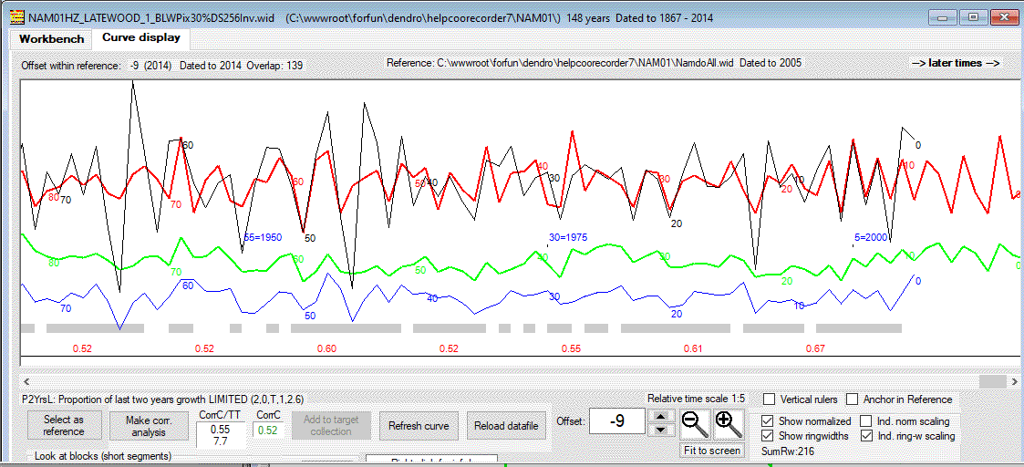
| We will set up two CI collectors. The first one is shown above. See that you have the same settings in CooRecorder. This first CI collector is set up to collect and save latewood inverted data which should crossdate towards ring widths. |
|
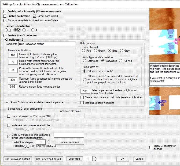
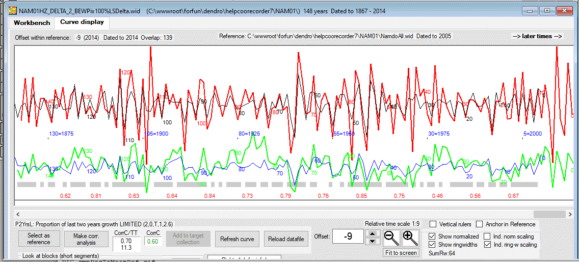
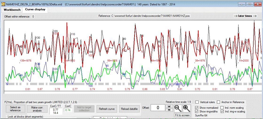
This is for the second CI collector which is set up to collect earlywood blue data for use to create a "delta-blue-file" as a difference
between this earlywood data and the latewood data collected by CI collector number 1.
To avoid having the curves diagram in our way, we close that window by unchecking the menu command "File/Enable ring width curve display (Ctrl-Tab)"
|
|
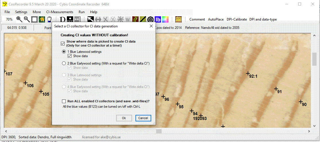
Click the blue "lb" icon! The window which popped up (above) is used in two alternative ways:
With the settings above, we click OK to start testing CI-collector number 1. |
|
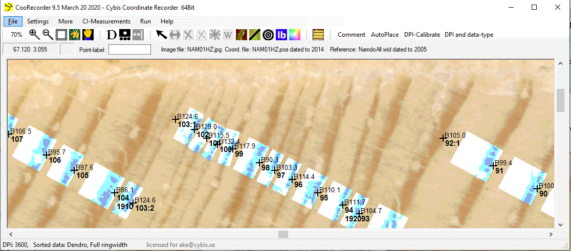
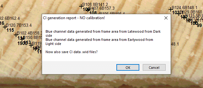
Blue areas are considered to be latewood. The dark blue areas are those selected for retrieving blue data. You have to scroll through the whole image and see that all blue areas are layed out correctly. When they are overlaying with a neighbour area you might have to (if possible) adjust the position of the ring border point (the numbered point). In case you want to save this latewood blue data, you have to click the menu command "File/Save CI measurement .wid files AND .pos file if unsaved" |
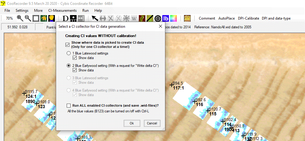
| To check also where the earlywood CI data is collected we once again click the blue lb icon and select CI collector number 2 as shown above and then click OK. |
| The blue areas in the picture above indicate where earlywood data is collected. Also in this case you have to look through the whole sample and see that there are no or few overlapping color spots. |
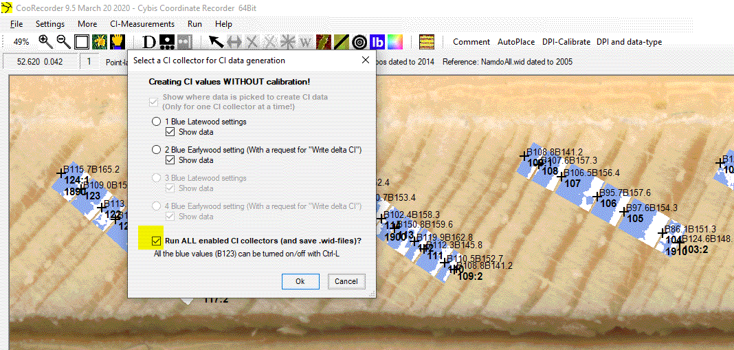
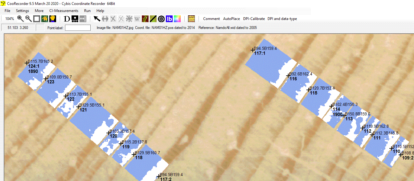
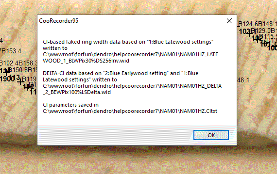
| Finally we again click the blue lb-icon and then check "Run ALL enabled CI collectors..." In this case the blue colored spots cannot be plotted as they would otherwise overwrite each other as we are running two CI collectors, one after the other. Click OK to start the calculations. |
Opening the files in CDendro
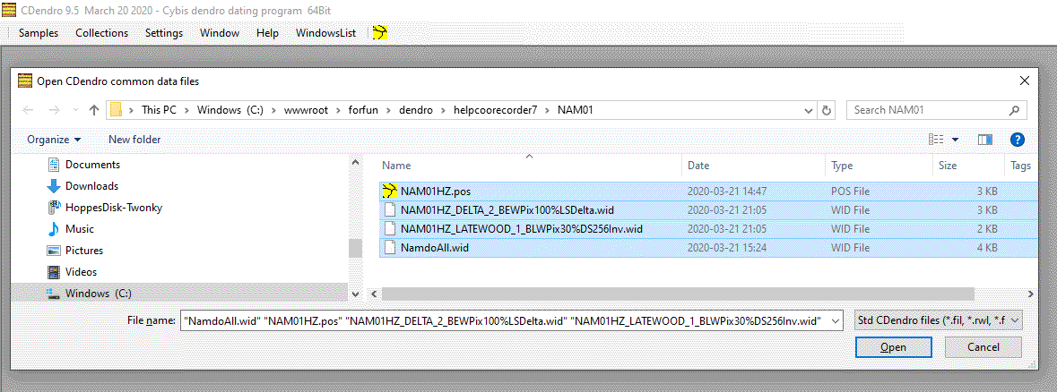
In CDendro, see that you open your three .wid files and also the .pos file.
Select NamdoAll.wid as your reference. (NamdoAll is a mean value of many detrended ring width samples)
|
What's next?
|
The intention with this lecture was to demonstrate how you can retrieve blue channel data with the help of CooRecorder. Hopefully you can now start to adjust parameters and thus experiment with other settings than those used above. If you are new to using CooRecorder, I recommend you to study all "help lectures" available at this site.
March 22 2020
|