Last update: 29 December 2015
|
This describes calibration and density measurements from an X-ray scanner image using CooRecorder version 8.1
|
|
 |
|
The output from an X-ray scanner is a gray-scale image where the variations in gray darkness correspond to variations in wood density.
Even with the old CooRecorder 7.8 you can measure these "gray shades" in the same way as you can measure "blue shades", though
you might have to first convert your gray scale image into an RGB color image. What is new with CooRecorder 8.0 is that you
can easily also transform (calibrate) the gray scale values into density values!
|
|
Calibrating the output of the X-ray scanner
|
 |
|
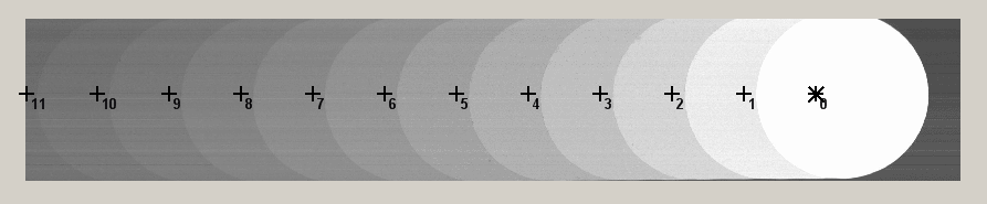
To calibrate your X-ray scanner you use a "standardized sample" ("a plexi ladder") as a "calibration target", which you scan with that scanner.
That scan gives you an image, the calibration image plexiladder.jpg,
where the different gray areas correspond to density values known in advance.
By measuring the gray shades of these areas with CooRecorder you get a "transformation table" (calibration curve) which (by interpolation) can be used
to convert gray scale values from actually scanned wood samples into wood density values.
This calibration - scanning of the plexi ladder - should possibly be done every day after the X-ray scanner has been
thoroughly warmed up. This means that you might get a new calibration image every day.
|
|
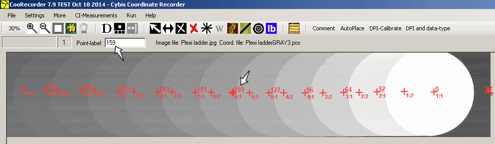 |
Defining the gray scale areas and binding a density value to each of them.
Each gray scale area should be marked
by "double-points" in CooRecorder, like 2:1, 2:2, 3:1, 3:2, 4:1, 4:2 etc. Because of the way CooRecorder works, the very first point has to be a single point not used
for calibration information - this is valid at least when the calibration file is of "dendro data type" and not of "raw type".
The "pair points" (.e.g. 3:1, 3:2) should all be placed on the border of an imaginary square so that each point is placed in the middle
of opposite sides of the square which then surrounds the corresponding gray scale region.
The "binding" of a density value to a certain gray scale region is done by storing a (scaled) density value like "127" into the point label for each double point at
its gray scale region.
With these points and point labels in place, you should save this as your "calibration file" e.g. as plexiladder.pos
(After you have used the command CI-Measurements/Create or load calibration curve and then Calibration CURVES/Create (X-Ray) calibration curve from ladder image .pos file
as described below you get a "calibration curve" that is also stored in a file.)
Note: This plexiladder.pos file can be opened with CooRecorder as the accompanying image file
plexiladder.jpg
is also available here.
Your selection of Data-type for the calibration file:
When the gray scale regions are all laying on a line one after the other on the calibration target, the data-type of the calibration image
when stored as a .pos file can very well be of type "Sorted data" like for a normal ring width coordinate file. Though if the regions are
distributed e.g. like on a chessboard, then "Type of data" should be set to one of the Raw data types, otherwise CooRecorder will complain
about "Erroneous order among points". In the case of raw type of datafile, the points will not be sorted in any order. Neither do you have
to care about the order as CooRecorder will automatically sort the gray shades for data conversion in the right way.
|
|
Checking the calibration file and creating a calibration curve
|
 |
|
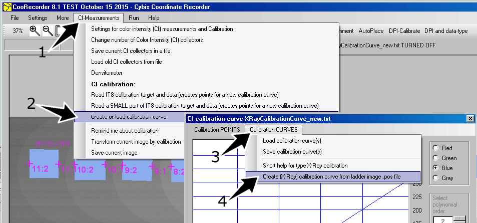
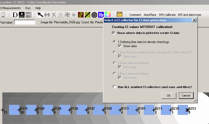
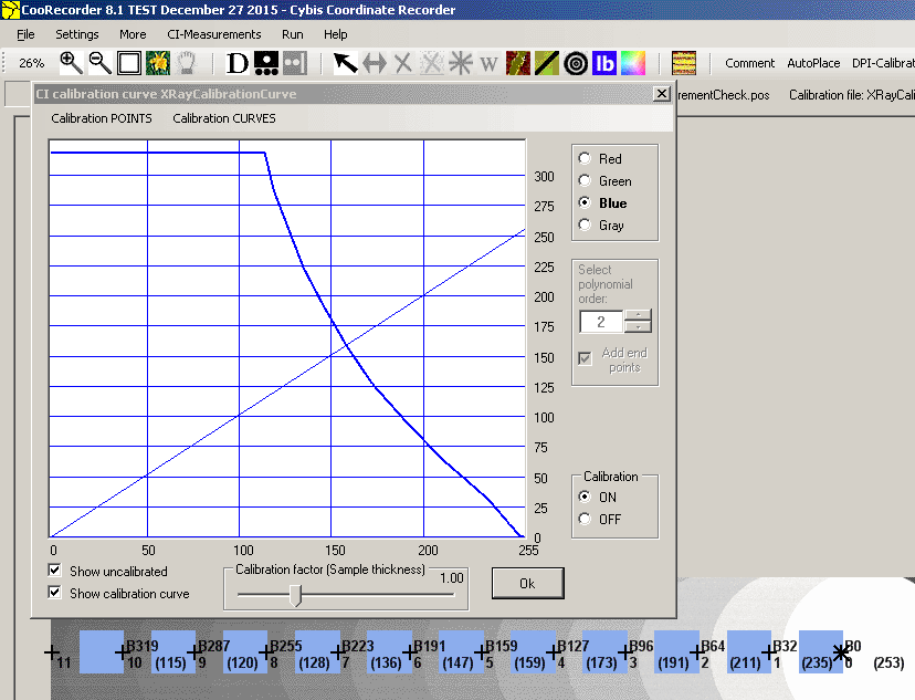
To create the "calibration curve" which will be used for calibrations, you should now issue the command "CI-measurements /Create or load calibration curve"
and then, within the window that pops up, "Calibration CURVES/Create(X-Ray) calibration curve from ladder image .pos file".
|
|
 |
|
This command will lay out the measurement frames from which the gray scale values (shades) will be calculated.
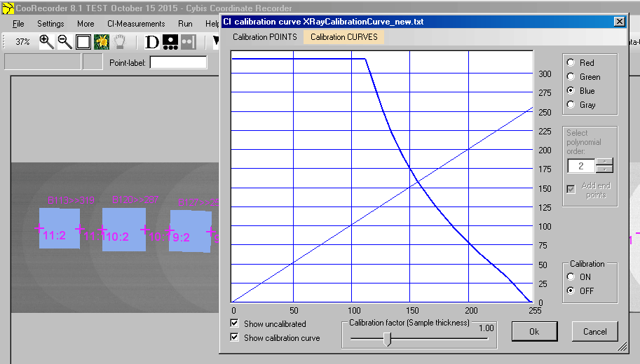
It will also check the consistency of the point-labels (describing known scaled density values for the various parts of the ladder) and create a "Calibration curve" as shown in the diagram above.
This curve will be used to transform gray scale values into densities when you later create CI data (blue lb-button) from the various gray shades of the X-ray scanned image of a wooden sample.
You should carefully inspect the calibration curve and how the the frames are laid out.
If you find errors, make your updates, save the file and see that you create a new calibration curve as described above.
When the calibration curve looks correct, see that you save it (Calibration CURVES/Save calibration curve(s)). The calibration curve is now loaded and ready to be used.
Though to have calibration actually turned ON, you have to see that the radiobutton for "Calibration ON" is checked, see in lower right corner above.
After you have closed the "CI calibration curve" window, you should also close the calibration image file.
Next time you want to use this calibration curve, use the command
CI-Measurements/Create or load calibration curve and then Calibration CURVES/Load calibration curve(s). And
again, do not forget to set the Calibration ON radiobutton before closing this window.
Now, to create calibrated density data, open an image or an already existing .pos file for which you want to generate density data.
Also see that you have a CI collector setup with a request to write data to a .wid file.
To actually create the density data, click the blue lb button and check the positions of all the frames showing from where the data is generated.
To save both your .pos file and the .wid-file(s) with density data use the command "File/Save CI measurement .wid file AND .pos file if unsaved"
|
|
 |
|
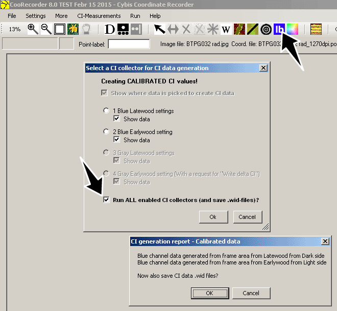
An even more easy way to quickly generate and save data for all enabled CI collectors is to check "Run ALL enabled CI collectors (and save .wid files)?"
and then click on OK for "Now also save CI data .wid files?" as shown above.
|
|
|
Remind me about calibration.
You can use the blue lb-button to create .wid files with either blue channel data or with density data.
To create density data you need to have a calibration curve "in use". If you have forgotten to do "CI measurents/Create or load calibration curve" and ,
within the window that then pops up, "Calibration CURVES/Load calibration curve(s)"
before you Calculate Color Intensity with the blue lb-button, you will get blue channel data and not density data which might make you confused.
With the command "Remind me about calibration" checked, you will be notified whenever you are doing an operation that should have been
preceded by the selection and usage of a calibration file. I.e. whenever you open a .pos file or you click the blue lb button to generate CI data.
|
|
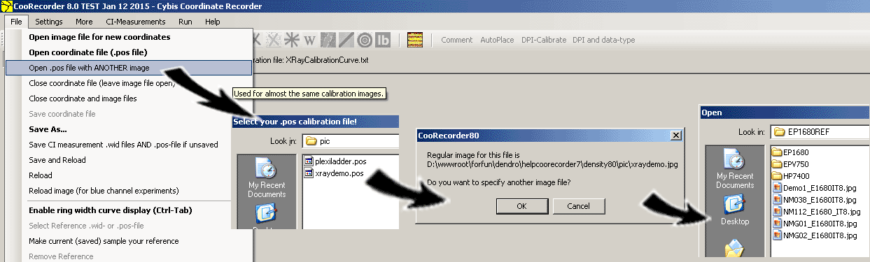
A new calibration file to measure in CooRecorder every morning?
How to facilitate?
|
 |
|
A scan of the calibration target (the "plexi ladder") should possibly be done every day after the X-ray scanner has been thoroughly warmed up.
So if you need to often recalibrate your scans by again scanning the calibration target, you might get tired of reentering points and density data
for your calibration image - which probably looks almost the same each time.
With the command "Open .pos file with ANOTHER image" you can replace the current image of a .pos file with another image.
I.e. if your calibration images always look almost the same though the gray shades might differ a little, you might replace the old image
of the .pos file with a new one. You then only have to check that the CooRecorder points are correctly placed and adjust if necessary
and then save the file (possibly with a new name) and finally order
the command CI-Measurements/Create or load calibration curve and then Calibration CURVES/Create (X-Ray) calibration curve from ladder image .pos file
This simple replacement of the .pos file image with a new one, might facilitate your calibration work considerably.
|
|
Checking your XRay/Density calibration
|
 |
|
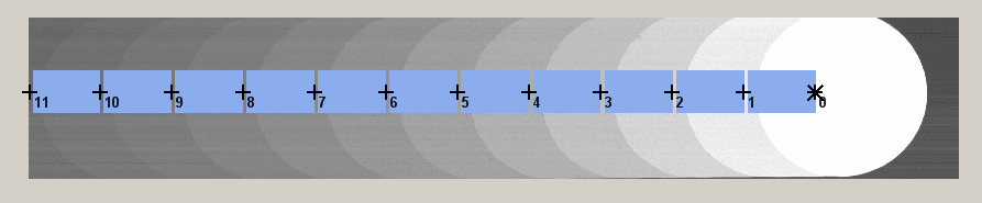
You can easily check your XRay/Density calibration by doing a measurement over that same "ladder image" that you used to create the XRay/density calibration curve.
In this case you set sort of ring border points in about the same way as when you measure ring widths on a wood sample.
|
|
 |
|
This is not the areas you want for your data collection!
In contrast to a wood sample where a new ring follows a previous ring you here have to limit the areas from where blue channel data is extracted.
|
|
 |
|
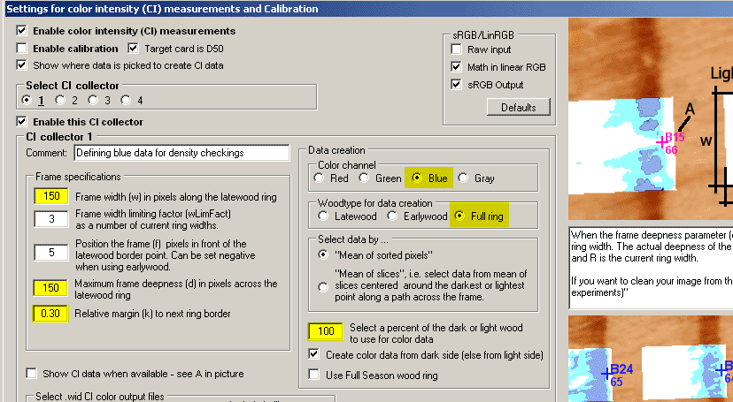
See that you limit the extension of your frames. The best value depends on the dpi resolution of your image. In this
case the image width is only 900 pixels, so I have selected the limits for the frames to 150 * 150 pixels.
Please note the Full ring and the Percentage settings!
|
|
 |
|
We now only have to load the XRay/Density calibration curve and also have calibration turned on.
You do this with the command CI-measurements/Create or load calibration curve and then within the
window that pops up, select Calibration CURVES/Load calibration curve and then select the calibration
curve you have earlier saved.
|
|
 |
|
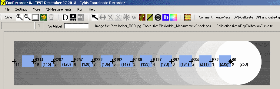
Your blue values will now be recalculated into density values according to your calibration curve.
As seen above the density values fully comply with the original labels set when the curve was created.
In this case the already calculated blue values for each "color spot" were converted to density values.
|
|
 |
|
If you again click on the blue lb-button the blue value reading and the calibration curversion will be done again.
This time every blue pixel value from within the "color spot" areas will be separately converted into a density value.
A mean density value can then be calculated for each spot.
These mean density values differ somewhat from the values
shown in the previous diagram. The biggest difference is for the leftmost spot where the requested value was
319 but the final value became 314.
So if we calculate a mean blue value for the whole spot and then convert
it to a density value, we then get 319. But if we convert every pixel's blue value into a density value and
then take the average value then we get 314! So this seems to be a matter of how we should calculate the density!
As the calibration curve is quite steep at this point the resulting density value will depend heavily on small changes within the blue color.
|
|